A Better Histogram
The photo-histogram is probably the most ubiquitous exposure tool in digital photography; that is, short light metering itself. It has been with us more than 25 years, and it hasn’t changed much. The histograms we are familiar with are calculated from transformed data, not raw data. Understanding how that transformation affects the resulting histogram can be important. Here we look at three kinds of photo-histograms: (1) the gamma level histogram, which is a transformed data histogram and is by far the most common type, (2) the linear level histogram, and (3) the stops histogram, which is the better histogram.
Understanding the dynamic range of image information, and how processing affects that dynamic range, is the key insight that histograms should inform.
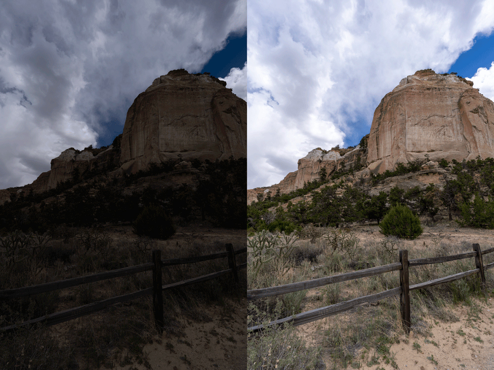
We’ll look at various histograms of Figure 1 images shot in the El Malpais National Monument in New Mexico. The image on the left is the unprocessed original. It is obviously underexposed, but it has a wide dynamic range most of which is lost in the deep shadow. The image on the right has been processed in the Lightroom Classic Develop module with a click of the auto-tone button. That did a bunch of stuff, like exposure = +1.96, contrast = +6, highlights = -75, … All histograms shown here were calculated from 16-bit ProPhoto TIFF files exported from Lightroom Classic.
The Standard Gamma Level Histogram
Even if you are a raw shooter, your camera and post software produce previews for display. That data has been transformed, in order of operation, by (1) transformation from the sensor’s native color space in linear color coordinates to linear RGB color channels, (2) application of the inverse Tone Rendering Curve (TRC) on each color channel, and (3) quantization (usually 8-bits).1 Every standard RGB space has its own TRC. Typically the TRC approximates the power law y = x? with ? ≈ 2.2, so I call this gamma level data.2
Linear data, on the other hand, is linearly related (in the mathematical sense) to the light intensity that strikes the sensor. Raw sensor data is essentially linear data.3
The data used for standard photo-histograms has been transformed by an inverse TRC. It is not linear data. TRCs are used solely because they improve quantization efficiency. That’s why JPEG and PSD files do so well with only 8 bit data, but linear raw data requires 12, 14 or even 16 bits.4
Figure 2 shows the standard gamma level histograms for the El Malpais images, except the labels on the horizontal axis are stops from full scale. The stop is the base two logarithm of the linear level (not the gamma level). That’s why the stops levels are distributed unevenly across the horizontal axis. Full scale white (on the right) is zero stops, and anything darker is negative stops.
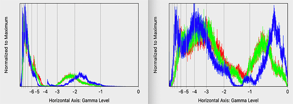
One of the things the stops labels show us is that this kind histogram is largely limited to 6 stops. Below that everything is squashed to the left. Six stops is not enough. We have cameras today that advertise 15 stops of dynamic range. Shouldn’t our data visualization tool be able to inform us of the entire dynamic range of the captured image?
The vertical scale is just awful! As is the usual practice, these histograms have been scaled so that their maximum values just touch the top of the drawing window.5 I call that normalized-to-max. That scaling will vary wildly for different images, or (as this example shows) different adjustments of the same image. The unprocessed image on the left has a very high but narrow peak below -6 stops that gets scaled down so much that it squashes the rest of the histogram. Post-processing pushes a lot of that ‘lost in the shadows’ information back into view above -6 stops, so we get an entirely different scaling on the right.
There is a better way! Scientists and engineers often use logarithmic scales because they allow visualization of data over several orders of magnitude. Log-scale charts are so ubiquitous that spread sheet programs such as Excel or Numbers offer log-scale charting with the click of a checkbox. Figure 3 shows the same gamma level histograms as in Figure 2, except with a log-vertical scale. The vertical axis now actually labeled with meaningful units: percent pixels per unit level. Moreover, it is the same scale on both histograms. Now we have a chance to do before/after comparisons! This is clearly a much better way to chart histograms, so all of the rest of the histograms shown here will use this log-scale vertical axis.
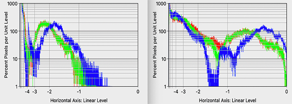
Linear Level Histograms
Histograms of linear level data, Figure 4, look similar to the gamma level histograms but notice that the stops from full-scale levels are even less evenly distributed than in the gamma level histograms. (That’s why standard RGB spaces use TRCs.) Whereas the gamma level histogram gave us good coverage for about six stops of dynamic range, here we only get about four stops. While interesting for technical reasons, this is clearly not the tool we need. So let’s move on.
The Stops Histogram
We deserve a data visualization tools that cover the dynamic range of modern digital cameras. Moreover, when we do an HDR merge, Lightroom Classic will produce a DNG file that stores the merged data in a floating-point digital format. Those files have a whopping 30 stops of potential dynamic range! See the DNG-HDR article. Thus, the gamma level histogram’s six effective stops is woefully inadequate. Human vision is limited to about 6.5 stops. That’s beside the point. The information below -6.5 stops from full scale is still useful image information, and processing can push it back into the range of our visual perception (as in the El Malpais images). The histogram thus needs to extend far below the 6.5 stops range of human vision.
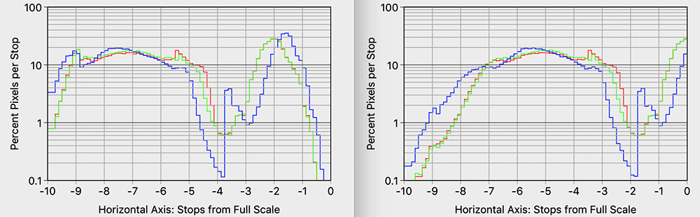
Of course, the answer is to use a log-scale on the horizontal axis. Of course, the photographer’s log-scale of choice is the base two logarithms that we call stops.
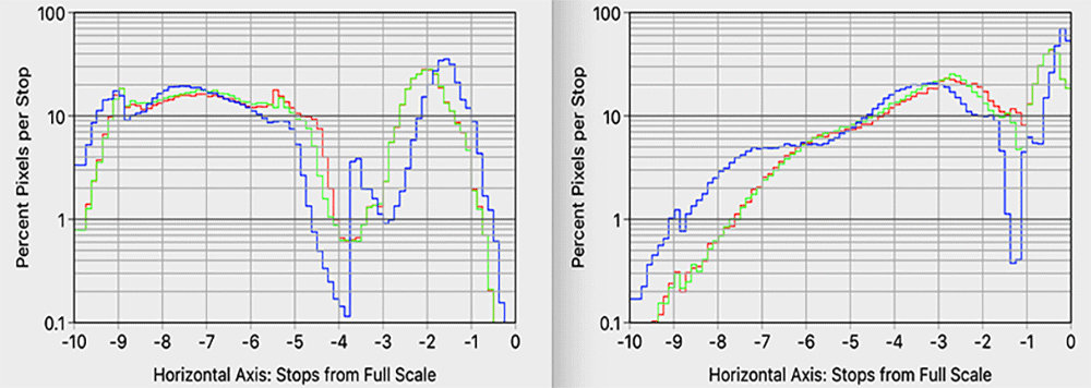
Point in Case: We should be able to make thumbnail estimates of where the data is from the histogram. From the left histogram in Figure 5 we see in the four stop range from -9 to -5 stops the histogram is between 10 to 20% per stop. So between 40 to 80% of all color channel values fall in this four-stop range. That’s a lot of data in the shadows. To my point, you could never make that kind of thumbnail analysis with a “normalized to max” gamma level histogram.
Discussions
Shape Stability
As we saw in Figure 2 that adjustments can cause wild changes in the standard histograms. A lot of that is due to the normalized-to-max vertical axis. Nonetheless, the shape of the histogram should be meaningful in some sense.
Consider this example. An exposure adjustment should have the effect of just shifting the histogram to the right without changing its shape. Figure 6 shows the El Malpais images: original (left) and processed only by a +2 stops true exposure adjustment (right).6 Precisely, that adjustment is a multiplier of 22 = 4 on linear data, followed by clipping. Anything above the -2 stops level in the unprocessed image will be clipped, which is shown in red on the right. Using my thumbnail percentage of pixels method on the left histogram of Figure 5, I estimate that ~15% of the pixels on the right side of Figure 6 are clipped.
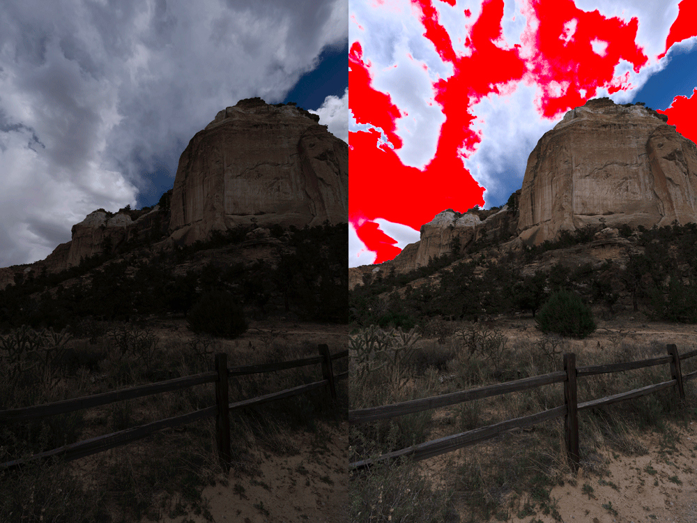
Figure 7 shows the resulting stops histograms. The ~15% clipped values are not shown here (they would be a large spike at zero stops), but we can clearly see the expected two-stop rightward shift. That’s what I mean by shape stability.
Historical Legacy
Things often are the way they are more due to legacy rather than what makes sense today. The reason for the widespread adoption of the gamma level histogram is fairly obvious. Cameras and post processing software calculate 8-bit sRGB gamma level preview images. The algorithm for calculating a histogram from this data needs to be simple and fast. So, initialize an array of 256 counters to zero, and then cycle through the color channel data using each the 8-bit value to select the counter to be incremented by one. After cycling through all the pixels we have an array of pixel counts, one count for each of the quantized gamma levels. Find the maximum, scale, draw, rinse and repeat. I call this the counter array algorithm. Given the much more limited processing power of the day, it makes perfect sense to use such a simple algorithm utilizing only the (smaller sized) preview data.
Smart Algorithms Lighten the Load
The histograms I’ve shown in this article were computed using a Mac application that I am currently developing. (If you are interested in being an alpha-tester, please contact me.) I experimented with several ways to calculate these histograms, and believe me, when you get into the details there are lot’s of ways to do this. I settled on an algorithmic scheme this is actually a modification of the counter array algorithm. I still use a counter array as the first step. The trick is to now interpret these counts relative to histogram “bins” in the linear and stops domains. Uniform width quantizer bins in gamma levels map to non-uniform bin widths in stops. So, I scale the histogram levels (divide by the bin width) for each linear or stops bin.
That’s about as succinctly as I can explain it without getting into mathematical notation and pseudo-code. The bottom line is that these algorithms are definitely not a burden for modern digital processing. I know, because I’ve implemented them.
Conclusions
Gamma levels are defined by the TRC of an RGB color space. In quantization theory, the inverse TRC is called a compressor function. The effect is that it changes the distribution of quantization levels so they more evenly distributed across the useful range of data values – not so heavily concentrated in the upper stops as with uniformly quantized raw data. Other than quantization efficiency, TRCs have no significant meaning, artistic or otherwise, for photography.
Yet gamma levels are used throughout our processing interfaces. In particular, curve adjustments are specified as gamma-to-gamma level bezier curves. Wouldn’t it be nice to have a bezier curve adjustment specified on a stops-to-stops scale, in conjunction with a stops histogram? How might that change the way we do HDR tone mapping.
Likewise, wouldn’t it be nice to have in-camera exposure tools based on raw image data stops levels rather than a TRC processed gamma histogram? Why do we use a gamma level in-camera histogram when we set exposure in stops?
The photographer’s logarithmic scale of choice is base 2 logarithm, the stop. That was established over a century ago, long before electronic imaging. We think in stops – not gamma levels. Our exposure and processing tools should likewise be stops base. I’ve shown that there is no computation problem for modern digital processing, as there once was. I understand that photographers are used to the standard “gamma level” histograms, and big changes are often difficult to swallow across an entire industry. This change, however, is well overdue.
End Notes
1. TRC is called a tone “rendering” curve because it renders the file data (gamma levels) back to the natural linear tones. Thus, it is the inverse TRC gets us from linear to gamma levels. For the power-law y = x? the inverse is x = y1/?.
2. In fact, the Adobe RGB TRC is exactly the power law with ? = 2.2.
3. It takes only a few tweaks (black point subtraction and linearization applied to the brightest levels) to yield true linear data from raw data. DNG files actually store “linear reference values.” See Chapter 5 of the DNG specification.
4. Historically, the TRC played another role as well. The only thing “special” about ? ≈ 2.2 is that CRT monitors from the 1990s had a power-law response with ? ≈ 2.2. sRGB data could drive CRT screens without additional color management. That was a big advantage at the time.
5. Histograms often do normalized-to-max separately on each color channel, so each channel has a different scale factor! I find that to be quite odd. Wouldn’t we want all three color channel histograms to be displayed on the same scale? In these histograms, I normalized to the maximum value over all three channels. Only the blue channel touches the top of the window.
6. I had to do this with an exposure adjustment layer in Photoshop. The Lightroom exposure slider is not a “true” exposure adjustment. It is actually a curve adjustment that is mostly linear but flattens at the top end so as not to push highlights into saturation as I have done in Figure 6. In my opinion, that Lightroom slider should be called brightness, or whatever. The term “exposure” should mean exactly the same thing as exposure in a camera.
John S. Sadowsky
November 2019
Charlestown, MD
John S. Sadowsky is a retired wireless system and signal processing engineer, with both academic and industrial experience. Now, I'm an amateur landscape photographer. I've done a lot of shooting in America's southwest, mostly in Arizona and southern Utah. Today I live in Maryland, where I'm learning to photograph an entirely different landscape.